Answer for Exam 1.1
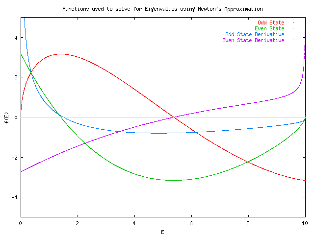
1.1.A. For the finite square well the energies eigenvalues are given by the
solutions to the equation beta*cos(alpha*a) - alpha*sin(alpha*a) = 0 for the
even states and alpha*cos(alpha*a) + beta*sin(alpha*a) = 0 for the odd
states. Alpha is given by sqrt(2mE/h^2) and beta is given by
sqrt(2m(V0-E)/h^2). For this example we took h^2/2m = 1, a=1 and V0=10. These
functions and their derivatives are plotted below. The eigenenergies of
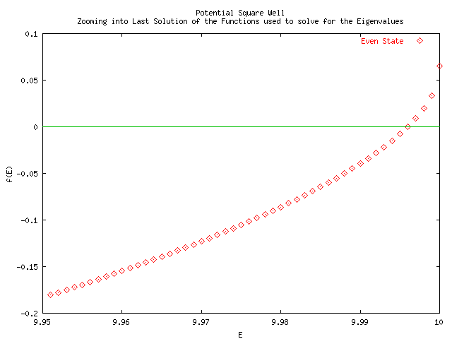
the three possible discrete states are given by E0 = 1.40721472477016, E1 =
5.37580591367022, and E2 = 9.99598073754667. These values were calculated
using an absolute precision so the computer could see no difference in the value
of the preceding term to the value of the current term. The calculation of
the 0th eigenenergy short-circuited at maxTries = 30,000.
1.1.B.
To evaluate the energy shifts we need to understand the following characteristics of the problem.
The following is a derivation of the equations needed to evaluate the first shift in the eigenenergy.
H = H0 + V’(x)
En = En0 + En’
H(psin) = Enpsin
psin = psin0 + S a’mnpsim0
H0 (psin) + V’(x) psin = (En0 + En’ )psin
En0 psin0 + H0 S a’mnpsim0 + V’(x) psin = En0 psin + En’psin
H0 S a’mnpsim0 + V’(x) psin = En0 S a’mnpsim0 + En’psin
V’(x) S a’mnpsim0 = En’ S a’mnpsim0 (keep only first order terms)
H0 S a’mnpsim0 + V’(x) psin0 = En0 S a’mnpsim0 + En’psin0
S a’mn Em0 psim0 + V’(x) psin0 = En0 S a’mnpsim0 + En’psin0
Applying the ket to both sides of the equation and using orthogonality
S a’nn En0 psin0 psin0 + psin0 V’(x) psin0 = En0 S a’nnpsin0 psin0 + psin0 En’psin0
psin0 V’(x) psin0 = psin0 En’psin0
En’ is constant in x so it can be taken out of the expectation value integration
En’ = < psin0 | V’(x) | psin0 > / < psin0 | psin0 >
1.1.C.
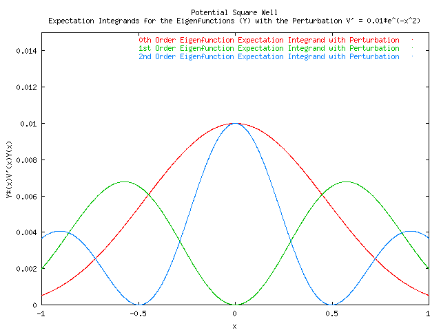
In order to achieve the integrations the eigenfunction psi was split up into three sections (-inf,-a) [-a,a] (a,inf). The expectation integral for the perturbing potential was evaluated in region 2 from [-a,a] because it was given as zero outside of this region. The expectation integral of the non-perturbed eigenfunctions was evaluated numerically inside of region 2, and analytically in region 1 and 3. The coefficients for the terms outside the well were evaluated based on the boundary value equation which allowed us to put the coefficient of these solutions in terms of the coefficient of the solution in region 2. This allowed for the cancellation of the coefficients, which made it unnecessary to normalize the eigenfunctions.
The expectation integrands in region 2 were calculated using romberg's approximation with a relative precision of 0.00000001.
The energy shifts were calculated as:
#Final Results
# E0 = 1.40721472477016 E0' = 0.0080335375623022 Tunneling Effect
=0.0480057645943113
# E1 = 5.37580591367022 E1' = 0.00551195218876488 Tunneling Effect
=0.249991679198193
# E2 = 9.99598073754667 E2' = 0.000435161775207359 Tunneling Effect
=15.7671147204421
The diminished effect of the perturbation on the second even eigenstate is due to the quantum tunneling effect which placed the probability of finding the particle outside of the well (in the classically forbidden region) at an amazing 94%.


//
//	This program evaluates the energy shifts for a square well perturbed by a potential
//
#include <functional>
#include <iostream>
#include <math.h>

using namespace std;

const double planks_constant = 7.6199682; // electron-mass * electron-volt * Angstrong^2

class Function : public unary_function<double,double>
{
public:
	Function() {};
	virtual result_type operator()(argument_type x){return x;};
	virtual Function& getDerivative() { return *this;};
};

class IdentityFunction : public Function
{
public:
	virtual double operator()(double x){return 1;};
};

class Approximation
{
public:
	Approximation(double lowerBound, double upperBound, Function& function)
		:a(lowerBound), b(upperBound), f(function)
	{};

	virtual double calculate(double precision, int maxTries = 3000)
	{
		cerr<< "Default approximation not implemented" << endl;
		return -1;
	}

protected:
	double a;
	double b;
	Function& f;
};

//calculates the zeros of a function using it's derivative
class NewtonApproximation : public Approximation
{
public:
	NewtonApproximation(double lower, double upper, Function& f, Function& derivative)
		:Approximation(lower,upper,f), d(derivative)
	{};
	double calculate(double precision=0.0, int maxTries=30000)
	{
		double x0 = (a+b)/2;
		double xn;
		double p = b-a;
		while ((p > precision) && (--maxTries))
		{
			//cout << "x=" << x0 << "\tf=" << f(x0) <<"\td=" << d(x0) << endl;
			xn = x0 - f(x0)/d(x0);
			if (xn>b) xn = (x0+b)/2;
			if (xn<a) xn = (x0+a)/2;
			p = fabs((x0-xn)/xn);
			x0=xn;
			//cout << p << endl;
		}
		if (!maxTries) cerr << "maxTries reached in Newton Approximation when value=" << xn << endl;
		return xn;
	};
protected:
};

//calculates the integral of a function
class RombergApproximation : public Approximation
{
public:
	RombergApproximation(double lowerBound, double upperBound, Function& function)
		:Approximation(lowerBound, upperBound, function)
	{};

	double calculate(double precision = 0.0, int maxTries = 25)
	{
		const int max_k = 5;
		double romberg[max_k][max_k];
		double i, sum0;
		int m = 1, k=1;
		double h = (b-a)/2;
		double sum = h*(f(a)+f(b))/2;
		romberg[0][0] = sum;

		if (h <= 0) return 0;
		do
		{
			double midpoints = 0;
			h/=2;m++;
			sum0 = sum;
			for (i = a+h; i < b; i+=2*h)
				midpoints +=f(i);
			sum =  sum0/2 + (b-a)*(midpoints)/pow(2,m);
			romberg[(m-1)%max_k][0] = sum;
			for (k=1;k< (( m < max_k) ? m : max_k);k++)
				romberg[(m-1)%max_k][k] =
				(pow(4,k)*romberg[(m-1)%max_k][k-1] - romberg[(m-2)%max_k][k-1])/(pow(4,k)-1);

			//cout << "# romberg[" << ((m-1)%max_k) << "][" << (k-1) << "] = " << romberg[(m-1)%max_k][k-1] << endl;;
			//cout << "# romberg[" << ((m-2)%max_k) << "][" << (k-2) << "] = " << romberg[(m-1)%max_k][k-2] << endl;;

		}  while ((fabs((romberg[(m-1)%max_k][k-1] - romberg[(m-2)%max_k][k-2])/
			romberg[(m-1)%max_k][k-1]) > precision) && (maxTries--));
		if (!maxTries) cerr << "# maxTries reached by romberg approximation accepting value : " << romberg[(m-1)%max_k][k-1] << endl;
		return romberg[(m-1)%max_k][k-1];
	};
};

// Defines a class of functions that represent a quantum square well eigenvalue problem.
class SquareWell : public Function
{
public:
	SquareWell() : d(0), a(1), V0(10), planks_square(planks_constant*planks_constant)
	{
		m = planks_square/2;
		getDerivative();
	};
	SquareWell(double potential_walls, double bound, double mass)
		: d(0), planks_square(planks_constant*planks_constant)
	{
		a = bound;
		V0 = potential_walls;
		m = mass;
		getDerivative();
	}
	virtual ~SquareWell()
	{
		if (d) delete d;
	};
	virtual double alpha(double E)
	{
		return sqrt(2*m*E/planks_square);
	};
	virtual double beta(double E)
	{
		return sqrt((V0 - E)*2*m/planks_square);
	}

protected:
	double a;
	double V0;
	const double planks_square;
	double m;
	Function* d;
};

// class used to solve for the eigenvalues
class EvenSquareWell  : public SquareWell
{
public:
	virtual double operator()(double E)
	{
		if (!d) //object is the derivative
			return (m/planks_square)*((-1/beta(E)- a) * cos(alpha(E)*a) -
				(1/alpha(E))*(1+a*beta(E))*sin(alpha(E)*a));
		else
			return beta(E)*cos(alpha(E)*a) - alpha(E)*sin(alpha(E)*a);
	};
	virtual Function& getDerivative()
	{
		if (!d)
			d = new EvenSquareWell(*this);
		return *d;
	}
};

class OddSquareWell : public SquareWell
{
public:
	virtual double operator()(double E)
	{
		//cout << "alpha=" << alpha << "\tbeta=" << beta << endl << ends;
		if (!d)
			return (m/planks_square)*((1+a*beta(E))*cos(alpha(E)*a)/alpha(E) -
				(1/beta(E) + a/alpha(E))*sin(alpha(E)*a));
		else
			return alpha(E)*cos(alpha(E)*a) + beta(E)*sin(alpha(E)*a);
	};
	virtual Function& getDerivative()
	{
		if (!d)
			d = new OddSquareWell(*this);
		return *d;
	}
};

//class used to evaluate the eigenfunction in the well (region 2)
class EigenFunc : public SquareWell
{
public:
	EigenFunc(int n, double eigenenergy) : En(eigenenergy), odd(n%2)
	{};
	virtual double operator()(double x)
	{
		if (odd)
			return sin(alpha(En)*x);
		return cos(alpha(En)*x);
	};
protected:
	double En;
	short odd;
};

//
//class used to evaluate the integrand of the expectation with a given perturbation
// <psi(x) | Perturbation(x) | psi(x) >
//
class ExpectationFunc : public Function
{
public:
	ExpectationFunc(EigenFunc& eigenfunc, Function& perturbation)
		: ef(eigenfunc), p(perturbation)
	{
	};
	virtual double operator()(double x)
	{
		return ef(x)*p(x)*ef(x);
	}

protected:
	EigenFunc& ef;
	Function& p;
};

// Represents the given perturbation V'(x) = e^(-x^2)
class Perturbation : public Function {
public:
	virtual double operator()(double x)	{return 0.01*exp(-x*x);}
};

// Calculates the solutions to the boundary condition derived equations
// that allow us to solve for the eigen values by approximating the zeros.
double eigenvalues(double lower, double upper, SquareWell& f)
{
	NewtonApproximation newtons(lower,upper, f, f.getDerivative());
	return newtons.calculate();
};

// This class will give the portion of the non-normalized expectation
//  outside the potential well up to a factor of B^2
class TunnelingEffect : public SquareWell
{
public:
	TunnelingEffect(int n) :_n(n) {};
	virtual double tunneling_coefficient(double E)
	{
		if (_n%2)
			//for odd state at x=a,  Asin(alpha*a) = Fe^(-beta*a)
			return sin(alpha(E)*a)*sin(alpha(E)*a)/exp(-2*beta(E)*a);
		else
			return cos(alpha(E)*a)*cos(alpha(E)*a)/exp(-2*beta(E)*a);
	};
	virtual double operator()(double E)
	{
		return 2*tunneling_coefficient(E)*(0.5/beta(E))*exp(-2.0*beta(E));
	};

protected:
	int _n;
};

//calculates the energy shifts for a given order eigen function and it;'s eigen value.
double energyshifts(int n, double En)
{
	double precision = 0.00000001;
	double perturbed,t,norm;
	IdentityFunction f;
	Perturbation p;
	TunnelingEffect tunneling_effect(n);
	EigenFunc ef(n, En);
	ExpectationFunc e(ef, f);
	ExpectationFunc ep(ef, p);

	cout << "# Position\t   Expectation Value  \t   Expectation with perturbation " << endl;
	for (double x = -1 ; x < 1; x+=.001)
		cout << x << "\t" << e(x) << "\t" << ep(x) << endl;
	RombergApproximation normalization_factor(-1,1, e);
	RombergApproximation perturbed_numerator(-1,1,ep);
	cout << "# perturbed : " << (perturbed = perturbed_numerator.calculate(precision)) << endl;
	cout << "# tunneling  : " << (t = tunneling_effect(En)) << endl;
	cout << "# normalize : " << (norm = normalization_factor.calculate(precision)) << endl;
	return  perturbed/(t+norm);
	//return perturbed_numerator.calculate(precision)/
	//	(2*tunneling_effect(En) + normalization_factor.calculate(precision));
};

void main (int argc, char* argv)
{
	const double e_step = 0.001;
	const double well_depth = 10;
	double E0,E1,E2, E0shift, E1shift, E2shift;
	OddSquareWell odd;
	EvenSquareWell even;
	TunnelingEffect tunneling0(0), tunneling1(1), tunneling2(2);
	cout.precision(15);
	cout << "# Welcome to the Square Well Quantum Problem with 1st-order Perturbation\n";
	cout << "# The solutions to the following data points represent the energy levels\n";
	cout << "\n#       E       \t         Odd State    \t       Even State\n";
	for (double E =e_step; E < well_depth; E+=e_step)
		cout << E << "\t" << odd(E) << "\t" << even(E) << "\t" << odd.getDerivative()(E) << "\t" << even.getDerivative()(E)<< endl;

	cout << "# The zero's of these function occur at:\n";
	cout << "# E0 = " << (E0 = eigenvalues(1,2, even)) << endl;
	cout << "# E1 = " << (E1 = eigenvalues(2,8, odd)) << endl;
	cout << "# E2 = " << (E2 = eigenvalues(9,9.9999999, even)) << endl;

	cout << "\n# The Romberg Integration Scheme yields the following results for the energy shifts\n";
	cout << "#  E0 = " << E0 << "\tE0' = " << (E0shift = energyshifts(0, E0)) << endl << endl;
	cout << "#  E1 = " << E1 << "\tE1' = " << (E1shift = energyshifts(1, E1)) << endl << endl;
	cout << "#  E2 = " << E2 << "\tE2' = " << (E2shift = energyshifts(2, E2)) << endl << endl;
	cout << "\n#Final Results\n";
	cout << "#  E0 = " << E0 << "\tE0' = " << E0shift << "\tTunneling Effect =" << tunneling0(E0) << endl;
	cout << "#  E1 = " << E1 << "\tE1' = " << E1shift << "\tTunneling Effect =" << tunneling1(E1) << endl;
	cout << "#  E2 = " << E2 << "\tE2' = " << E2shift << "\tTunneling Effect =" << tunneling2(E2) << endl;
};
#Final Results
#  E0 = 1.40721472477016	E0' = 0.0080335375623022	Tunneling Effect =0.0480057645943113
#  E1 = 5.37580591367022	E1' = 0.00551195218876488	Tunneling Effect =0.249991679198193
#  E2 = 9.99598073754667	E2' = 0.000435161775207359	Tunneling Effect =15.7671147204421


# perturbed : 0.0107741008609386
# tunneling  : 0.0480057645943113
# normalize : 1.29313452103734

# Chances of particle being in the well 0.964205262410933016251385682648323

#  E0 = 1.40721472477016	E0' = 0.0080335375623022

# perturbed : 0.00807518122913154
# tunneling  : 0.249991679198193
# normalize : 1.21503939374749

# Chances of particle being in the well 0.829360834855506435027570601590505

#  E1 = 5.37580591367022	E1' = 0.00551195218876488

# perturbed : 0.00729916622643665
# tunneling  : 15.7671147204421
# normalize : 1.00633975624884

# Chances of particle being in the well 0.0599959750477929148195148422826652

#  E2 = 9.99598073754667	E2' = 0.000435161775207359
Bibliography
Blatt, Frank. J. (1992) Modern Physics (McGraw-Hill: NY), pp. 140-147.
Devries, Paul ( 1993) A First Course in Computational Physics (John Wiley & Sons: NY), pp. 74-83, 155-156.
Liboff, Richard. L (1991) Introductory Quantum Mechanics Second Edition. (Addison Wesley: NY), Ch. 8 &13.
Merzbacher, Eugen (1988) Quantum Mechanics Third Edition. (John Wiley & Sons: NY).
Shankar, R. (1994) Principals of Quantum Mechanics Second Edition. (Plenum Press: NY).
Discussion of the Bibliography
1.. Blatt, Frank. J. (1992) Modern Physics (McGraw-Hill: NY), pp. 140-147. QC21.2.B56 1992 Elementary discussion of a particle in a one dimensional square well.
2. Devries, Paul ( 1993) A First Course in Computational Physics (John Wiley & Sons: NY), pp. 74-83 discuss the square well and pp 155-156 discuss the Romberg Integration Scheme. .
3. Liboff, Richard. L (1991) Introductory Quantum Mechanics Second Edition. (Addison Wesley: NY), Ch. 8 &13.
4. Merzbacher, Eugen (1988) Quantum Mechanics Third Edition. (John Wiley & Sons: NY). pp. 92-93, 103-111, 128, 142-146, 452-459 & Problem 8.4. Contains a lot of background information that is helpful with the understanding of this problem.
5. Arfken, George (1985) Mathematical Methods for Physicists Third Edition. (Academic Press Inc)
6. Shankar, R. (1994) Principals of Quantum Mechanics Second Edition (Plenum Press: NY). QC174.12.S52