Answer for Problem 3.1
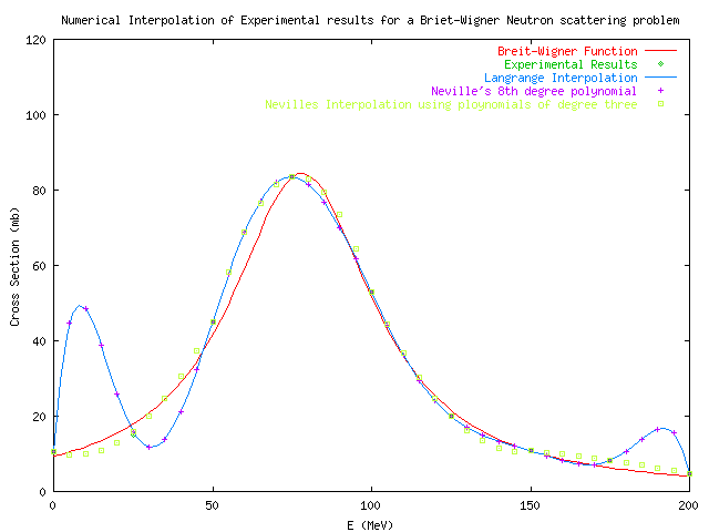
The plot below shows the function representing the cross section for a neutron beam scattering experiment which measures the cross section of the scattering for a neutron beam of a given energy blasts it's nucleus. Using the data given, a standard Neville Interpolation was performed on the data, as well as a Lagrange Interpolation 9th order polynomial, and the most successful of the algorithms, Neville's Interpolation using polynomials of degree three to achieve LOCAL curve fitting.

Data was generated using nevilles.cpp. This file contains a simple recursive function to calculate the value of a function at a given x using data points to interpolate a value at that x. As can be seen from the graph, The 8th order polynomial that was evaluated in the first loop gave some very large deviations from the actual Breit-Wigner curve. The second loop was designed to use only three points at a time to interpolate the polynomial. This gave a much closer fit. It was shown that higher order polynomials introduce inaccuracy into an interpolation.
It is obvious from the graph that using third degree polynomials reduced the error in the interpolation. These points were used to determine the resonant energy and the width of the resonance peak at half height by averaging the solutions of the simultaneous equations given by our interpolated points. The Breit-Wagner function is given as:
cross section= initial cross section / ( ( energy of incoming beam-energy of the resonance ) ^ 2 + resonance width ^ 2 / 4 )
Where initial cross section is assumed to be 6.389x10⁴. Although the actual equation gave the values Energy of resonance = 78, and resonance width = 55, the technique used (averaging out of solution to simultaneous equations) gave values of 85.1348 for the energy of resonance and 63.9752 for the width at half height of the resonance process. In order to verify the algorithm, the solution was bracketed around the peak. This brought the average values much closer to the desired result. At the extremes of the function there is very little change, and insignificant error could sway the solutions to simultaneous equations. Potentially a Monte Carlo, or least squares method might be useful in place of the arithmetic mean. Many of the simultaneous equations derived from the interpolated data did not have a solution. These terms needed to be dropped. The equation is given below.
resonance width = sqrt ( initial cross section / cross section - (energy of beam - energy of resonance) ^2) )
energy of resonance = 1/2 * ( (initial cross section) * (1 / cross section ( i ) - 1 / cross section( i + 1)) - (energy of beam ( i ) ^ 2 + energy of beam ( i + 1 ) ^ 2 ) ) / (energy of beam ( i+1 ) + energy of beam ( i ) )
g(x)=10.6*((x-25)/-25)*((x-50)/-50)*((x-75)/-75)*((x-100)/-100)*((x-125)/-125)*((x-150)/-150)*((x-175)/-175)*((x-200)/-200)\
 + 16*((x)/25)*((x-50)/(25-50))*((x-75)/(25-75))*((x-100)/(25-100))*((x-125)/(25-125))*((x-150)/(25-150))*((x-175)/(25-175))*((x-200)/(25-200))\
 + 45*(x/50)*((x-25)/(50-25))*((x-75)/(50-75))*((x-100)/(50-100))*((x-125)/(50-125))*((x-150)/(50-150))*((x-175)/(50-175))*((x-200)/(50-200))\
 + 83.5*(x/75)*((x-25)/(75-25))*((x-50)/(75-50))*((x-100)/(75-100))*((x-125)/(75-125))*((x-150)/(75-150))*((x-175)/(75-175))*((x-200)/(75-200))\
 + 52.8*(x/100)*((x-25)/(100-25))*((x-50)/(100-50))*((x-75)/(100-75))*((x-125)/(100-125))*((x-150)/(100-150))*((x-175)/(100-175))*((x-200)/(100-200))\
 + 19.9*(x/125)*((x-25)/(125-25))*((x-50)/(125-50))*((x-75)/(125-75))*((x-100)/(125-100))*((x-150)/(125-150))*((x-175)/(125-175))*((x-200)/(125-200))\
 + 10.8*(x/150)*((x-25)/(150-25))*((x-50)/(150-50))*((x-75)/(150-75))*((x-100)/(150-100))*((x-125)/(150-125))*((x-175)/(150-175))*((x-200)/(150-200))\
 + 8.25*(x/175)*((x-25)/(175-25))*((x-50)/(175-50))*((x-75)/(175-75))*((x-100)/(175-100))*((x-125)/(175-125))*((x-150)/(175-150))*((x-200)/(175-200))\
 + 4.7*(x/200)*((x-25)/(200-25))*((x-50)/(200-50))*((x-75)/(200-75))*((x-100)/(200-100))*((x-125)/(200-125))*((x-150)/(200-150))*((x-175)/(200-175))
set xlabel "E (MeV)"
set ylabel "Cross Section (mb)"
set title "Numerical Interpolation of Experimental results for a Briet-Wigner Neutron scattering problem"
plot [x=0:200] [0:120] 63890/((x - 78)*(x-78) + 55*55/4) title "Breit-Wigner Function", "interdata.txt" using 1:2 title "Experimental Results", g(x) title "Langrange Interpolation",  "nevillesdata.txt" every :::0::0 using 1:2 title "Neville's 8th degree polynomial", "nevillesdata.txt" every :::1::1 using 1:2 title "Nevilles Interpolation using ploynomials of degree three"
nevilles.cpp
#include <iostream.h>
#include <math.h>
double nevilles(double x, double *data, double * f, int lower, int upper)
{
	int a=lower-1;
	int b=upper-1;
	//cout << a << "," << b << endl;
	if (a==b) return f[a];
	return (x-data[b])/(data[a]-data[b]) *nevilles(x, data, f, lower, upper-1) +
		(x-data[a])/(data[b]-data[a]) *nevilles(x, data, f, lower+1, upper);
}
int main (int argc,char* argv[])
{
	const int num_of_values = 9;
	double data[num_of_values] = {0,25,50,75, 100,125,150,175,200};
	double  values[num_of_values] = {10.6, 16.0, 45.0, 83.5, 52.8, 19.9, 10.8, 8.25, 4.7};
	int inc =3;
	int i, j, k,m;
	double x, y, average_x=0, average_y=0;
	//double x ;
	//while (1)
	//{
		cout << "# Welcome to the Nevilles Interpolation Alogrithm program" << endl;
		//cout << "# These are the data points" << endl;
		//for (int i=0;i<num_of_values;i++)
		//	cout << "# " << data[i] << "\t" << values[i] << endl;
		//cout << "# Please enter an x value to interpolate : ";
		//cin >> x;
		//cout << "# The nevilles algorithm interpolated value is " << nevilles(x, data, values, 1, num_of_values) << endl;
	//}
	for (i = 0; i <= 200; i+=5)
		cout << i << "\t" << nevilles(i, data, values, 1, num_of_values) << endl;
cout << endl;
	for (i=0, j = inc, k=0,m=0 ;i <= 200; i+=5, k++,m++)
	{
		cout << i << "\t" << nevilles(i, data, values, j -inc+1, j) << endl;
		if (i >= data[j-1] )  j+=inc-1;
	}
	for (i=0, j = inc, k=0;i <= 200; i+=5)
	{
		double value = nevilles(i, data, values, j -inc+1, j);
		for (int i2=i+5, j2 = j; ((i2 <= 200) && (j2<=num_of_values)); i2+=5)
		{
			double  inner_value = nevilles(i2, data, values, j2 -inc+1, j2);
			x = (63890*(1/value - 1/inner_value) - (i)*(i) +i2*i2)/(2*(i2-i));
			if ((63890/value - (x-i)*(x-i)) > 0)
			{
				y = 2*sqrt(63890/value - (x-i)*(x-i));
				average_x +=  x;
				average_y += y;
				k++;
				//cout << x  << "\t" << y << endl;
			}
			if (i2 >=data[j2-1]) j2+=inc-1;
		}
		if (i >= data[j-1] )  j+=inc-1;
	}
	cout << "# Average Energy : " << average_x/(k) << endl;
	cout << "# Average cross section: " << average_y/(k) << endl;
	return 0;
}
# Welcome to the Nevilles Interpolation Alogrithm program
0	10.6
5	44.8336
10	48.581
15	38.7101
20	25.8487
25	16
30	11.8688
35	13.9312
40	21.2793
45	32.269
50	45
55	57.6522
60	68.7035
65	77.0495
70	82.0473
75	83.5
80	81.5988
85	76.8384
90	69.9177
95	61.6368
100	52.8
105	44.1324
110	36.2148
115	29.442
120	24.0052
125	19.9
130	16.9565
135	14.8904
140	13.3677
145	12.0769
150	10.8
155	9.47062
160	8.2075
165	7.30863
170	7.18987
175	8.25
180	10.6424
185	13.9317
190	16.6117
195	15.4598
200	4.7
0	10.6
5	9.792
10	9.928
15	11.008
20	13.032
25	16
30	19.912
35	24.768
40	30.568
45	37.312
50	45
55	58.236
60	68.704
65	76.404
70	81.336
75	83.5
80	82.896
85	79.524
90	73.384
95	64.476
100	52.8
105	44.316
110	36.784
115	30.204
120	24.576
125	19.9
130	16.176
135	13.404
140	11.584
145	10.716
150	10.8
155	10.37
160	9.9
165	9.39
170	8.84
175	8.25
180	7.62
185	6.95
190	6.24
195	5.49
200	4.7
# Average Energy : 85.1348
# Average cross section: 63.9752