Abdul Khan
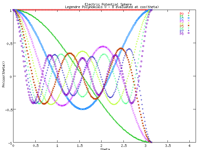
Given a sphere with a potential defined on it's surface as V(theta) = e^(-cos^2(theta)), and the general solution for the potential inside the sphere is given by V(theta) = SUMn(0,inf)(An*r^n*Pn(cos(theta))), we can plot this potential using algorithms to find the values of the Legendre polynomials. In addition we can use the boundary condition to find the coefficients (An)s = (2n+1)/2a^n * integral(0,pi)( V(theta)*Pn(cos(theta))*sin(theta) dtheta ).

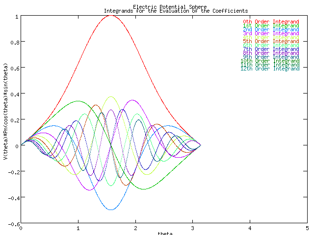
These are the integrands used to evaluate the coefficients plotted below. It was noticed that the integrand for the odd orders was an odd function function centered at pi/2. This made it obvious that the coefficient would be zero. It allowed for a much needed performance boost.
We plotted 2000 coefficients noticing that the alternating series seemed to be converging, and the differences between the positive and negative terms were growing increasingly small. To generate these numbers the precision of the approximation was less than the following plot of coefficients from 0 to 200. The same pattern was obvious.
.
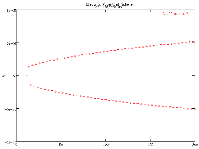
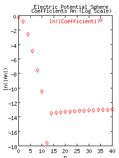
If we look at the first 20 coefficients evaluated using a single precision Romberg approximation (relative error = 1.0e-8) we see that in fact our approximation seems to converge to 0 until the 12th coefficient, after which there is what could be an expression of error within the numerical approximation.
# The coefficients (An) are given by
|
|
This could be the nature of the problem though, so in order to insure
single precision accuracy the relative error of the total potential was
evaluated and compared at every other significant coefficient. The
iteration was halted when the relative error of these totals was less than
1.0e-8. The plots for the coefficient that resulted in giving such a
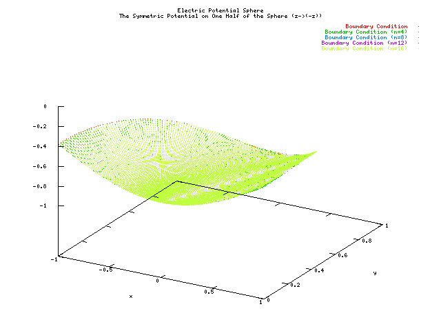
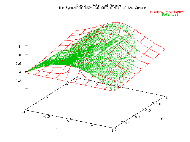
relative error were then generated giving us the spherical potential in one half
the sphere (0<theta<pi). Because of symmetry this was sufficient to
realize the correct answer. 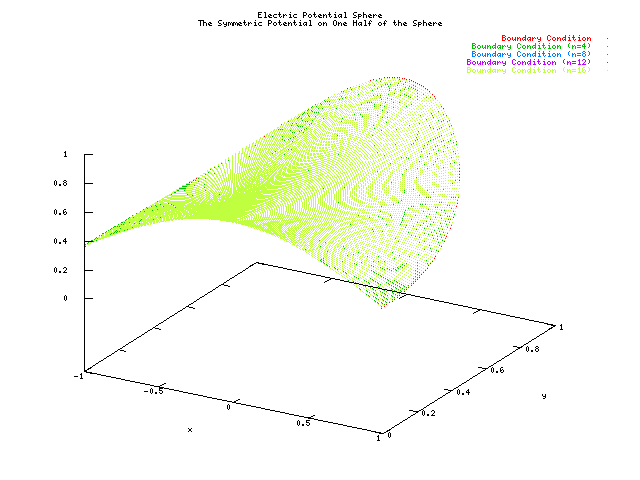
legendre.cpp
//
// This program calculates the potential inside a sphere whose potential is given on the surface using Legendre polynomials.
//

#include <functional>
#include <vector>
#include <iostream>
#include <time.h>
#include <math.h>

using namespace std;

const double zero = 0.0;
const double pi = acos(-1);
const double nan = 1/zero;
const double e = exp(1);

//
// The following group of classes were an attempt to develop a way to call functions on functions
//
class Function : public unary_function<double,double>
{
public:
	Function() {};
	virtual ~Function()
	{
		//do garbage collection on tempFunctions //crashes program?
		for (vector<Function*>::iterator  iter = tempFunctions.begin(); iter != tempFunctions.end(); iter++)
			delete *iter;
	};
	virtual double operator()(double x){return x;};
	virtual Function& operator^(Function& f);
	virtual Function& operator*(Function& f);
	virtual Function& operator+(Function& f);
	virtual Function& operator-(Function& f);
	virtual Function& operator()(Function& f);

	virtual Function& operator^(double x);
	virtual Function& operator*(double x);
	virtual Function& operator+(double x);
	virtual Function& operator-(double x);

	virtual Function& operator-();

	virtual Function& getDerivative() { return *this;};
protected:
	 vector<Function*> tempFunctions;
};


class PowFunc : public Function
{
public:
	PowFunc(Function&f1, Function& f2) : a(f1), b(f2) {}
	virtual double operator() ( double x) { return pow(a(x),b(x));};
	virtual Function& getDerivative();

protected:
	Function& a;
	Function& b;
};

Function& Function::operator^(Function& f)
{
	PowFunc* a;
	tempFunctions.insert(tempFunctions.end(), (a = new PowFunc(*this, f)));
	return *a;
};

Function& PowFunc::getDerivative()
{
	cerr << "can not evaluate f(x)^g(x).  Need to develop numerical approximation" <<endl;
	return a*b;
};


class AdditionFunc : public Function
{
public:
	AdditionFunc(Function&f1, Function& f2) : a(f1), b(f2) {}
	virtual double operator() ( double x) { return (a(x)+b(x));};
	virtual Function& getDerivative();
protected:
	Function& a;
	Function& b;
};

Function& Function::operator+(Function& f)
{
	AdditionFunc* a;
	tempFunctions.insert(tempFunctions.end(), (a = new AdditionFunc(*this, f)));
	return *a;
};

Function& AdditionFunc::getDerivative()
{
	return (a.getDerivative() + b.getDerivative());
};

class SubtractionFunc : public Function
{
public:
	SubtractionFunc(Function&f1, Function& f2) : a(f1), b(f2) {}
	virtual double operator() ( double x) { return (a(x)-b(x));};
	virtual Function& getDerivative();

protected:
	Function& a;
	Function& b;
};

Function& Function::operator-(Function& f)
{
	SubtractionFunc* s;
	tempFunctions.insert(tempFunctions.end(), (s = new SubtractionFunc(*this, f)));
	return *s;
};

Function& SubtractionFunc::getDerivative()
{
	return (a.getDerivative() - b.getDerivative());
};

class MultiplyFunc : public Function
{
public:
	MultiplyFunc(Function& f1, Function& f2) :a(f1), b(f2) {};
	virtual double operator() ( double x) { return a(x)*b(x);};
	virtual Function& getDerivative();

protected:
	Function& a;
	Function& b;
};

Function& Function::operator*(Function& f)
{
	MultiplyFunc * m;
	tempFunctions.insert(tempFunctions.end(), (m = new MultiplyFunc(*this, f)));
	return *m;
};

Function& MultiplyFunc::getDerivative()
{
	return (a.getDerivative()*b + a*b.getDerivative());
};

class CompositionFunc : public Function
{
public:
	CompositionFunc(Function& f1, Function& f2) :a(f1), b(f2) {};
	virtual double operator() ( double x) { return a(b(x));};
	virtual Function& getDerivative();
protected:
	Function& a;
	Function& b;
};

Function& Function::operator()(Function& f)
{
	CompositionFunc* c;
	tempFunctions.insert(tempFunctions.end(), (c = new CompositionFunc(*this, f)));
	return *c;
};

Function& CompositionFunc::getDerivative()
{
	return (a.getDerivative()(b)*b.getDerivative());
};

class ConstFunc : public Function
{
public:
	ConstFunc(double x) : _x(x) {};
	virtual double operator()(double x){return _x;};
protected:
	double _x;
};

class IdentityFunction : public ConstFunc
{
public:
	IdentityFunction() : ConstFunc(1) {};
};

class VectorFunc : public Function
{
public:
	VectorFunc(vector<double> &list) : v(list) {};
	virtual double operator()(double n) { return v[(int)n]; };
protected:
	vector<double> & v;
};

IdentityFunction identityFunc;

Function& Function::operator^(double x)
{
	ConstFunc* c;
	tempFunctions.insert(tempFunctions.end(), (c = new ConstFunc(x)));
	return ((*this)^(*c));
}
Function& Function::operator*(double x)
{
	ConstFunc* c;
	tempFunctions.insert(tempFunctions.end(), (c = new ConstFunc(x)));
	return ((*this)*(*c));
};
Function& Function::operator+(double x)
{
	ConstFunc* c;
	tempFunctions.insert(tempFunctions.end(), (c = new ConstFunc(x)));
	return ((*this)+(*c));
}
;
Function& Function::operator-(double x)
{
	ConstFunc* c;
	tempFunctions.insert(tempFunctions.end(), (c = new ConstFunc(x)));
	return ((*this)-(*c));
}
;
Function& Function::operator-()
{
	ConstFunc* c;
	tempFunctions.insert(tempFunctions.end(), (c = new ConstFunc(0)));
	return ((*c) - (*this));
};

//time to move this to a header file
#define functor(NAME, FUNC) \
class NAME : public Function \
{\
public: \
	virtual Function&  operator()(Function& x) { return Function::operator ()(x);}; \
	virtual double operator()(double x) { return FUNC(x);}; \
};

#define FunctionObject(FUNCTION) \
	functor(FunctionObject##FUNCTION, FUNCTION) \
	FunctionObject##FUNCTION FUNCTION##F;

#define FunctionObjectSpec(NAME, FUNCTION, OBJECT) \
	functor(NAME,FUNCTION) \
		NAME OBJECT;\

#define FunctionObjectSpecPtr(NAME, FUNCTION, OBJECT) \
	functor(NAME,FUNCTION) \
		NAME* OBJECT;\


#define FunctionObject_(NAME, FUNCTION) \
	functor(NAME,FUNCTION) \
	NAME FUNCTION##F;

FunctionObjectSpec(ExponentialFunc, exp, exponentialFunc);

FunctionObjectSpec(CosFunc, cos, cosFunc)

FunctionObjectSpec(SinFunc, sin, sinFunc);

class SumFunc : public Function
{
public:
	enum Type {Int, Dub};
	SumFunc(int lower, int upper, int increment = 1) : a(lower), b(upper), inc(increment), type(Int) {};
	SumFunc(double lower, double upper, double increment = 1) : a(lower), b(upper), inc(increment), type(Dub){};
	virtual double operator()(double x) { return ((b-a)/inc)*x; };
	virtual Function& operator()(Function& f)
	{
		double val = 0;
		for (double n = a;n<=b;n+=inc)
			val += f(n);
		ConstFunc *c = new ConstFunc(val);
		tempFunctions.insert(tempFunctions.end(), c);
		return *c;
	};


protected:
	double a, b, inc;
	Type type;
};


//
//	This body of code was developed to find the potential inside a sphere where the
//  potential on the surface is given
//

class Legendre : public Function
{
public:
	Legendre(int coefficient_num) : n(coefficient_num), nmax(0), gotAll(nan){};
	Legendre(int coefficient_num, int maxN) : n(coefficient_num), nmax(maxN), gotAll(nan){	};
	virtual Function&  operator()(Function& x) { return Function::operator ()(x);};
	virtual double operator()(double x)
	{
		if (!n) return 1;
		if (!nmax)
		{
			int i;
			double pn = 1;
			double pn1 = x;
			for (i=1;i<n;i++)
			{
				double pn2 = 2*x*pn1 - pn - (x*pn1 - pn)/(i+1);
				pn = pn1;
				pn1 = pn2;
			}
			return pn1;
		}
		if (gotAll != x)
		{
			int tmp = n;
			n = nmax;
			getAll(x);
			n = tmp;
		}
		return vals[n];
	};
	virtual vector<double> getAll(double x)
	{
		vals.insert(vals.end(), 1);
		vals.insert(vals.end(),x);
		for (int i=1;i<n;i++)
		{
			double pn = vals[i-1];
			double pn1 = vals[i];
			vals.insert(vals.end(), 2*x*pn1 - pn - (x*pn1 - pn)/(i+1));
		}
		gotAll = x;
		return vals;
	}
	virtual double lastX() {return gotAll;};
	virtual vector<double> getValues() {return vals;};
	virtual int getN() { return n;};
protected:
	int n;
	int nmax;
	vector<double> vals;
	double gotAll;
	};


class Approximation
{
public:
	Approximation(double lowerBound, double upperBound, Function& function)
		:a(lowerBound), b(upperBound), f(function)
	{};

	virtual double calculate(double precision = 0.1, int maxTries = 3000)
	{
		cerr<< "Default approximation not implemented" << endl;
		return -1;
	}

protected:
	double a;
	double b;
	Function& f;
};


//calculates the integral of a function
class RombergApproximation : public Approximation
{
public:
	RombergApproximation(double lowerBound, double upperBound, Function& function)
		:Approximation(lowerBound, upperBound, function)
	{};

	double calculate(double precision = 0.0, int maxTries = 20)
	{
		const int max_k = 5;
		double romberg[max_k][max_k];
		double i, sum0;
		int m = 1, k=1;
		double h = (b-a)/2;
		double sum = h*(f(a)+f(b))/2;
		romberg[0][0] = sum;

		if (h <= 0) return 0;
		do
		{
			double midpoints = 0;
			h/=2;m++;
			sum0 = sum;
			for (i = a+h; i < b; i+=2*h)
				midpoints += f(i);
			sum =  sum0/2 + (b-a)*(midpoints)/pow(2,m);
			romberg[(m-1)%max_k][0] = sum;
			for (k=1;k< (( m < max_k) ? m : max_k);k++)
				romberg[(m-1)%max_k][k] = (pow(4,k)*romberg[(m-1)%max_k][k-1] - romberg[(m-2)%max_k][k-1])/(pow(4,k)-1);
			//cout << "# romberg[" << ((m-1)%max_k) << "][" << (k-1) << "] = " << romberg[(m-1)%max_k][k-1] << endl;;
			//cout << "# romberg[" << ((m-2)%max_k) << "][" << (k-2) << "] = " << romberg[(m-1)%max_k][k-2] << endl;;
		}  while ((fabs((romberg[(m-1)%max_k][k-1] - romberg[(m-2)%max_k][k-2])/romberg[(m-1)%max_k][k-1]) > precision) && (maxTries--));
		if (!maxTries) cerr << "maxTries reached for romberg integration resulting in value " << romberg[(m-1)%max_k][k-1]<< endl;
		return romberg[(m-1)%max_k][k-1];
	};
};

double coefficient(int n, double r, Approximation& integration, double precision)
{
	if (n%2) return 0; //speed improvment An for odd n was integration of odd function
	return (((2*(double)n) + 1)/(2*pow(r,n)))*integration.calculate(precision, 20);
};

class RombergCoefficient : public Function
{
public:
	RombergCoefficient(double radius,  double precision) : r(radius), p(precision) {};
	virtual double operator()(double n)
	{
		Legendre legendre(n);
		ConstFunc eVal(e);
		Function potential = (eVal^(-(cosFunc^2)));
		RombergApproximation romberg(0,pi, (potential*(legendre(cosFunc))*sinFunc));
		return coefficient((int)n, r, romberg, p);
	};
protected:
	double p;
	double r;
};


void main(int argc, char*argv[])
{
	const int maxCoefficient =200, maxCinc=3;
	const int maxPlotCoefficient = 20;
	const double r_inc = 0.01;
	const double theta_inc = .005*pi;
	const double rombergPrecision = 0.00000001;
	int i, maxC;
	double theta, r;
	time_t t0,t1,t2,t3,t4;

	ConstFunc eVal(e);
	Function& potential = (eVal^(-(cosFunc^2)));

	cout. precision(15);
	cout << "# Welcome to the Legendre Polynomial Example using a Sphere with Potential \n";
	cout << "# V(theta) = e^(-cos^2theta)\n";
	cout << "# We know that the potential inside the sphere can be written as\n";
	cout << "# Potential(r,theta) = sumn(0, infinity, An*(r^n)*Pn(cos(theta))\n";

	cout << "# The Integrand of the coefficient formula and the value of the Legendre Poynomial is given by \n";
	t0 = time(0);
	for (theta = 0; theta <= pi ; theta+=theta_inc)
	{
		cout << theta << "\t";
		Legendre legendre(maxCoefficient);
		vector<double> pn = legendre.getAll(cos(theta));
		for (i = 0; i <= maxPlotCoefficient; i++)
		{
			Legendre legendre(i);
			cout  << (double) (potential*legendre(cosFunc)*sinFunc)(theta) << "\t";
			cout << pn[i] << "\t";
			//cout << (exp(-cos(theta)*cos(theta))*sin(theta)*pn[i]) << "\t";
		};
		cout << endl;
	};
	cout << "# Calculation of these Integrand points took " << ((t1=time(0))-t0) << " seconds" << endl;

	cout << "\n# The coefficients (An) are given by\n";
	vector<double> coefficients(maxCoefficient);
	for (i = 0;i<=maxCoefficient;i+=2)
	{
		Legendre legendre(i);
		RombergApproximation romberg(0,pi, (potential*(legendre(cosFunc))*sinFunc));
		cout << i << "\t" << (coefficients[i] = coefficient(i, 1, romberg, rombergPrecision)) << endl;
	};
	cout << "#Calculation of the coefficients took " << ((t2=time(0))-t1) << endl;

	double potentialT = 0, pT = .01, oldp = 1, prevp = 2;
	//loop until the realitve error of the sum of all the calculated points of the potential is single precision
	for (maxC = 2; (fabs(pT - oldp)/pT > 0.00000001) && (maxC <= maxCoefficient); maxC+=2)
	{
	oldp = prevp; prevp = pT; pT=0;  //alternating series so test relative error comparing every other term
	for (theta=0; theta <= pi; theta= theta + theta_inc)
	{
		Legendre legendre(maxCoefficient);
		vector<double> pn = legendre.getAll(cos(theta));
		for (r=0.;r<=1.;r = r + (float)r_inc)
		{
				FunctionObject(exp);
				for (i=0, potentialT=0;i<=maxC;i+=2)
				{
					potentialT += coefficients[i]*pow(r, i)*pn[i];
				};
				pT+=potentialT;
		}
	}
	cout << "#\n# The sum of all the potential values for the " << maxC << " approximation is " << pT << endl;
	cout << "# The absolute error is " << pT-oldp << " and the relative error is " << (pT-oldp)/pT << endl;
	cout << "# Calculation of the potential for " << maxC << " coefficients took " << ((t3=time(0))-t2) << endl;
	}
	cout << "#\n# The potential inside the sphere is defined by the following points\n#theta\tr\tPotential\n";

	for (theta=0; theta <= pi; theta= theta + theta_inc)
	{
		Legendre legendre(maxCoefficient);
		vector<double> pn = legendre.getAll(cos(theta));
		for (r=0.;r<=1.;r += r_inc)
		{
				FunctionObject(exp);
				for (i=0, potentialT=0;i<=maxC;i+=2)
				{
					potentialT += coefficients[i]*pow(r, i)*pn[i];
				};
				cout << theta << "\t" << r << "\t" << potentialT << endl;
		}
	}


	//The whole algorithm can be written in terms of Function objects as seen below.
	//This led to an approximately 30% increase in the time necessary to make the calculations
	/*
	for (int maxC = 2; (fabs(pT - oldp)/pT > 0.00000001) && (maxC <= maxCoefficient); maxC+=2)
	{
	for (theta=0; theta <= pi; theta+= theta_inc)
	{
		Legendre legendre(maxCoefficient);
		vector<double> pn = legendre.getAll(cos(theta));
		for (r=0.;r<=1;r += r_inc)
		{
				FunctionObject(exp);
				FunctionObjectSpec(SelfFunction, 1*,selfF);
				SumFunc sumFunc(0, maxC);
				RombergCoefficient rombergCoefficient(1, rombergPrecision);
				VectorFunc legendreVals(pn);
				VectorFunc coefficientVals(coefficients);
				ConstFunc radius(r);

				cout << maxC << "\t";
				double potential = sumFunc(coefficientVals*(radius^selfF)*legendreVals)(0);
				cout << theta << "\t" << r  << "\t" << potential << "\t";
				if (r > 1 - r_inc) cout << (expF(-(cosFunc^2))(theta)) << "\t";
				cout << endl;
		}
	}
	cout << "# Calculation of the potential for " << maxC << " coefficients using function objects took " << ((t4=time(0))-t3) << endl << endl;
	}
	*/
};
Output of Program
Errata
The relative error of the sum of all the plotted potential points did not represent the actual error of the system because the sum of the points was much larger than their differences. The same algorithm as above was used after replacing the break from the maxC loop with the absolute error (fabs(pT-oldp)). The file legendrefix.cpp contains the code necessary to complete these calculations, and the file legendredatafixold.txt represents the output of a very similar version of the program. If anyone feels like running it and plotting the relative and absolute error as a function of the number of coefficients to a gif file, I would be happy to include it in this errata. My computer is tired, and there are still a couple hours left of spring break. Regardless, from the data it can be seen that the number of coefficients needed to achieve single precision absolute error for 20,000 points is 294.