Electrostatic Potential

Answer for Assignment 5

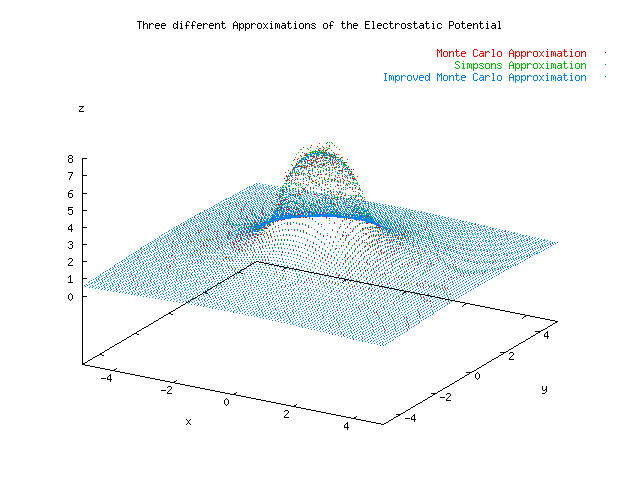
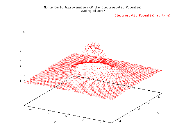
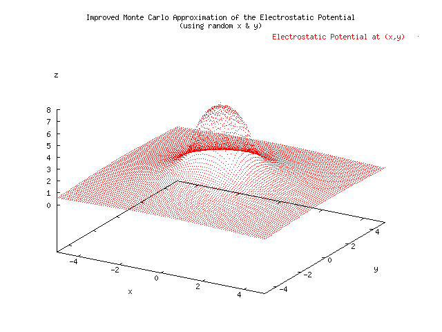
Below is a plot showing the results of three different approximations for the electrostatic potential given a uniform charge density located x=[-1,1], y=[-1,1]. A Monte Carlo estimate was able to achieve 0.005 precision, where 1/sqrt(N) was take to be the error, in 676 seconds. The Simpson's Approximation had a hard time reaching a precision of 0.005, and at the borders of the charge distribution had to short circuit using a max number of iterations set to 20. This method took 1210 seconds, almost twice as long. The error was measured using the relative difference of the current computation with the previous computation. The slice integration technique was not suitable for the MonteCarlo Approximation because it reduced the randomness of the samples by choosing N random x's and evaluating N random y's for each of those x's. An improved MonteCarloApproximation which did not rely on slicing was developed. The increased randomness of the variables seems to have reduced the error in the graph. The speed was increased to 244 seconds, almost five times as fast as the Simpson's Approximation. .

electrostatic.cpp

/*
Function
	MultiDFunc
		ElectrostaticFunc-------\
				template|-------> ApproxFunc<Approximation, MultiDimensionalFunc>
	SimpsonsApproximation-----------/
	MonteCarlo---------------------/
Approximation

The class hierarchy above demonstrates the use of templates and inheritance to create a generic solution for solving multi dimensional integral approximations where n-one dimensions are held constant through a recursive call to the Approximation function calculate() and the Function operator (). This can be thought of as a type of slicing integration method.

The beauty of the pattern can be found in the fact that the Approximation class uses the Function class to calculate it's value. It is itself a function, but should not need knowledge of a particular function. ApproxFunc uses virtual inheritance to re-implement the Approximation's calculate function to recursively call Approximation's calculate until all the n-1 dimensional approximations have been stored on the stack. It then sets a member variable for that iteration of the Approximation's to return actual values, beginning the unwinding of the stack to achieve a n dimensional calculation.

The ugliness of the pattern is found by over-dependence on the slice integral where it may not be smart to apply as can be seen by examining the improved MonteCarloApproximation.

*/

#include <functional>
#include <iostream>
#include <math.h>
#include <vector>
#include <stdlib.h>
#include <time.h>

using namespace std;

const double zero = 0.0;
const double nan = 1/zero;
const double pi = acos(-1);
const double minDouble = 	0.00000000000001;

//
//  ApproxFunc is a template class that represents both a function and an approximation
//  It is a generic solution to performing multidimensional approximations using a recursive 
// algorithm.
//
template <class approx, class multiDFunc>
class ApproxFunc : public approx, public multiDFunc
{
public:
	ApproxFunc(double lowerBound, double upperBound, multiDFunc* function, int dimensions=2)	
		: approx(lowerBound, upperBound,function), multiDFunc(*function),  current_d(dimensions), store_vals(1)
	{
		f=this;
		if (a >=b) cerr << "Lowerbound " << a << " is greater than or equal to upper bound " << b << endl;
	};
	virtual double calculate()
	{
		double ret;
		if (current_d == 1)
		{
			store_vals=0;
			ret = approx::calculate();
			store_vals=1;
		}
		else
		{
			current_d--;
			ret =  approx::calculate();
			current_d++;
		}
		return ret;
	}
	virtual double operator()(double x_)
	{
		if (store_vals)
		{
			x[current_d-1]=x_;
			return calculate();
		}
		else 
		{
			return multiDFunc::operator ()(x_);
		}
	};
protected:
	int current_d;
	int store_vals;
};

class Function : public unary_function<double,double>
{
public:
	Function() {};
	virtual double operator()(double x){ return x;};
	virtual Function& getDerivative() { return *this;};
};

//
//  MultiDFunction is used as a base class for functions that wish to be incorporated into
//  the ApproxFunc template.  It stores a vector of double values that represent chosen
// points in the previous dimensions of the recursion.   These are available during the
// actual calculation of a point.
//
class MultiDFunction :public Function
{
public:
	MultiDFunction(int dimension) :x(d-1), d(dimension) {};
	virtual double operator()(double x, double y, ...) = 0;
	~MultiDFunction() {};
protected:
	int d; 
	vector<double> x;
};

class ElectrostaticPotential: public MultiDFunction
{
public:
	ElectrostaticPotential(double at_x, double at_y, double singularAvoidance = minDouble)
		: xp(at_x), yp(at_y), sinc(singularAvoidance), MultiDFunction(2) 
	{};
	ElectrostaticPotential(const ElectrostaticPotential& ep)
		: xp(ep.get_xp()), yp(ep.get_yp()), sinc(ep.get_singularAvoidance()), MultiDFunction(2)
	{};
	virtual double operator()(double val)
	{
		if ((fabs(x[0] - xp) < sinc) && (fabs(val-yp) < sinc)) 
			return  1/(sqrt(2)*sinc); //top off singularities //nan;  
		return sqrt(1/((x[0]-xp)*(x[0]-xp)+(val-yp)*(val-yp)));
	};
	virtual double operator()(double x, double y, ...)
	{
		if ((fabs(x - xp) < sinc) && (fabs(y-yp) < sinc)) 
		{
			cerr << "singularity found in ElectrostaticFunction at (" << x << "," << y << ")" << endl;
			return  1/(sqrt(2)*sinc); //top off singularities //nan;  
		}
		return sqrt(1/((x-xp)*(x-xp)+(y-yp)*(y-yp)));
	};

	double get_xp() const {return xp;};
	double get_yp() const {return yp;};
	double get_singularAvoidance() const {return sinc;};
protected:
	double xp;
	double yp;
	double sinc;
};

class Approximation
{
public:
	Approximation(double lowerBound, double upperBound, Function* function)
		:a(lowerBound), b(upperBound), f(function)
	{};

	virtual double calculate(double precision=0, int maxTries = 3000)
	{
		cerr << "Default approximation not implemented" << endl;
		return -1;
	}
protected:
	double a;
	double b;
	Function* f;
	//TBD: set precision & maxTries?
};

class MonteCarlo : public Approximation
{
public:
	MonteCarlo(double lowerBound, double upperBound, Function * function)	
		: Approximation(lowerBound, upperBound,function)
	{
		if (a >=b) cerr << "Lowerbound " << a << " is greater than or equal to upper bound " << b << endl;
	};

	virtual double calculate(double precision=0.07, int maxTries = 300000)
	{
		double sum=0, val;
		double r;
		double n;
		double N = 1/(precision*precision);
		double randmult = (b-a)/RAND_MAX;

		for (n=0;n < N;n++)
		{
			r = rand()*randmult;
			//cerr << n << "\t" << r << endl; //test quality of random number generator
			val = (*f)(r+a);
			if (val == nan)
			{
				n--;
				cerr << "Monte Carlo got  NAN (" << (*(ElectrostaticPotential*)f).get_xp() << "," << (*(ElectrostaticPotential*)f).get_yp() << ") " << endl;
			}
			else sum += val;
		}
		return (sum/n)*(b-a);
	}
};

class SimpsonsApproximation : public Approximation
{
public:
	SimpsonsApproximation(double lowerBound, double upperBound, Function* function)	
		: Approximation(lowerBound, upperBound,function)
	{
		if (a >=b) cerr << "Lowerbound " << a << " is greater than or equal to upper bound " << b << endl;
	};

	virtual double calculate(double precision=0.005, int maxTries=20)
	{
		if (b<=a+precision) return 0;
		double i, sum0, val, val0;
		double h = (b-a)/3;
		double se= val0 = (*f)(a+2*h),	so = (*f)(a+h) + (*f)(b-h),	sd = (*f)(a) + (*f)(b);

		double sum;

		double singularAvoidance = (b-a)/(3 * pow(2,maxTries));
		while ((so == nan) || (se==nan) || (sd == nan))
		{ 
			//cerr << "Modifying bounds" << endl;
			a += singularAvoidance;
			b -= singularAvoidance;
			h = (b-a)/3;
			se= val0 = (*f)(a+2*h);
			so = (*f)(a+h) + (*f)(b-h);
			sd = (*f)(a) + (*f)(b);
		}

		sum = h*(sd + 2*se + 4*so)/3;

		do 
		{
			h/=2;
			sum0 = sum;
			se+=so;
			so =0;
			for (i = a+h; i < b; i+=2*h)
			{
				val = (*f)(i);
				if (val == nan)
				{
					so+= (val = val0);
					//cerr << "Function returned NAN for i =" << i << " at (" << (*(ElectrostaticPotential*)f).get_xp() << "," << (*(ElectrostaticPotential*)f).get_yp() << ")" << endl;
				}
				else
					so += (val0=val);
			}
			sum =  h*(sd  + 2*se +4*so)/3;
			//cout << sd << "\t" << se << "\t" << so << "\t" << sum << endl;
		}  while ((fabs((sum - sum0)/sum0) > precision) && (--maxTries));
		if (!maxTries) 
			cerr << "maxTries reached at (" << (*(ElectrostaticPotential*)f).get_xp() << "," << (*(ElectrostaticPotential*)f).get_yp() << ") with precision = "  <<
				fabs((sum - sum0)/sum0)  << endl << " and sum = " << sum <<endl ;
		return sum;
	}
};

class MonteCarlo2dApproximation : public Approximation
{
public:
		MonteCarlo2dApproximation(double lowerBound, double upperBound, MultiDFunction* function)	
		: Approximation(lowerBound, upperBound,function)
	{
		if (a >=b) cerr << "Lowerbound " << a << " is greater than or equal to upper bound " << b << endl;
	};

	virtual double calculate(double precision =0.005, int maxTries=-1)
	{
		double total = 0;
		double N = 1/(precision*precision);
		double randmult = (b-a)/RAND_MAX;
		for (int i=0;i<N;i++)
				total += (*(MultiDFunction*)f)((a+rand()*randmult), (a+rand()*randmult));

	return total*(b-a)*(b-a)/(N);
	};
};

int main(int argc, char* argv[])
{
	double inc = 0.1, montesinc=0.0000005,simpsonssinc=0.0000005, x, y;
	unsigned long t0,t1,t2,t3;

	//cout.precision(10);

	cout << "# Welcome to the Electrostatic Potential Integration using the Monte Carlo Technique" << endl;
	cout << "# Current Time : " << (t0  =  time(0)) << endl;
	cout << endl;

	cout << "# Monte Carlo" << endl;
	for (x=-5.0;x<=5.0;x+=inc)
	{
		for (y=-5.0;y<=5.0;y+=inc)
		{		
			ElectrostaticPotential *f = new ElectrostaticPotential(x,y);
			ApproxFunc<MonteCarlo, ElectrostaticPotential> full_integral(-1.0,1.0, f);
			cout << x << "\t" << y <<"\t" << full_integral.calculate() <<endl;
			delete f;
		}
	};
	cout << "# Monte Carlo ApproxFunc ended at : " << (t1 = time(0)) << endl;

	
	cout << endl << "# 2-D Simpson Approximation" << endl;
	for (x=-5.0;x<=5.0;x+=inc)
	{
		for (y=-5.0;y<=5.0;y+=inc)
		{		
			ElectrostaticPotential *f = new ElectrostaticPotential(x,y,simpsonssinc);	
			ApproxFunc<SimpsonsApproximation, ElectrostaticPotential> full_integral(-1.0,1.0, f);
			cout << x << "\t" << y <<"\t" << full_integral.calculate() <<endl;
			delete f;
		};
	};
	cout << "# Simpsons ApproxFunc ended at : " << (t2 = time(0)) << endl;

	cout <<  endl << "# Monte Carlo Approximation" << endl;
	for (x=-5.0;x<=5.0;x+=inc)
	{
		for (y=-5.0;y<=5.0;y+=inc)
		{		
			ElectrostaticPotential *f = new ElectrostaticPotential(x,y,montesinc);
			MonteCarlo2dApproximation full_integral(-1.0,1.0, f);
			cout << x << "\t" << y <<"\t" << full_integral.calculate(0.005) <<endl;
			delete f;
		}
	};
	cout << endl << "# Execution completed at time : " << (t3 = time(0)) << endl << endl;

	cout <<endl << "# MonteCarlo ApproxFunc: " << (t1 -t0) << endl;
	cout << "# Simpsons ApproxFunc: " << (t2 - t1) << endl;
	cout << "# MonteCarlApproximation : " << (t3 - t2) << endl;

	return 0;
};

electrostaticplot.txt

electrostaticdata.txt

Time for each approximation:

# MonteCarlo ApproxFunc: 676

# Simpsons ApproxFunc: 1210

# MonteCarlApproximation : 244